6 Conditional expectation
6.1 Conditional mean
Conditional expectation
The conditional expectation or conditional mean of Y given \boldsymbol Z= \boldsymbol b is the expected value of the distribution F_{Y|\boldsymbol Z=\boldsymbol b}: E[Y | \boldsymbol Z= \boldsymbol b] = \int_{-\infty}^\infty a \ \text{d}F_{Y|\boldsymbol Z = \boldsymbol b}(a).
For continuous Y with conditional density f_{Y|\boldsymbol Z = \boldsymbol b}(a), we have \text{d}F_{Y|\boldsymbol Z = \boldsymbol b}(a) = f_{Y|\boldsymbol Z = \boldsymbol b}(a) \ \text{d}a, and the conditional expectation is E[Y | Z= \boldsymbol b] = \int_{-\infty}^\infty a f_{Y|\boldsymbol Z = \boldsymbol b}(a)\ \text{d}a. Similarly, for discrete Y with support \mathcal Y and conditional PMF \pi_{Y|\boldsymbol Z = \boldsymbol b}(a), we have E[Y | Z= \boldsymbol b] = \sum_{u \in \mathcal Y} u \pi_{Y|\boldsymbol Z = \boldsymbol b}(u).
The conditional expectation is a function of \boldsymbol b, which is a specific value of \boldsymbol Z that we condition on. Therefore, we call it the conditional expectation function: m(\boldsymbol b) = E[Y | Z= \boldsymbol b].
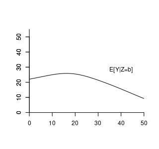
Suppose the conditional expectation of wage given experience level b is: m(b) = E[wage | exper = b] = 14.5 + 0.9 b - 0.017 b^2. For example, with 10 years of experience: m(10) = E[wage | exper = 10] = 21.8.
Here, m(b) assigns a specific real number to each fixed value of b; it is a deterministic function derived from the joint distribution of wage and experience.
However, if we treat experience as a random variable, the conditional expectation becomes: \begin{align*} m(exper) = E[wage | exper] = 14.5 + 0.9 exper - 0.017 exper^2. \end{align*} Now, m(exper) is a function of the random variable experexper and is itself a random variable.
In general:
- The conditional expectation given a specific value b is: m(\boldsymbol b) = E[Y | \boldsymbol Z=\boldsymbol b], which is deterministic.
- The conditional expectation given the random variable Z is:
m(\boldsymbol Z) = E[Y | \boldsymbol Z],
which is a random variable because it depends on the random vector \boldsymbol Z.
This distinction highlights that the conditional expectation can be either a specific number, i.e. E[Y | \boldsymbol Z=\boldsymbol b], or a random variable, i.e., E[Y | \boldsymbol Z], depending on whether the condition is fixed or random.
6.2 Rules of calculation
Let Y be a random variable and \boldsymbol{Z} a random vector. The rules of calculation rules below are fundamental tools for working with conditional expectations:
(i) Law of Iterated Expectations (LIE):
E[E[Y | \boldsymbol{Z}]] = E[Y].
Intuition: The LIE tells us that if we first compute the expected value of Y given each possible outcome of \boldsymbol{Z}, and then average those expected values over all possible values of \boldsymbol{Z}, we end up with the overall expected value of Y. It’s like calculating the average outcome across all scenarios by considering each scenario’s average separately.
More generally, for any two random vectors \boldsymbol{Z} and \boldsymbol{Z}^*:
E[E[Y | \boldsymbol{Z}, \boldsymbol{Z}^*] | \boldsymbol{Z}] = E[Y | \boldsymbol{Z}].
Intuition: Even if we condition on additional information \boldsymbol{Z}^*, averaging over \boldsymbol{Z}^* while keeping \boldsymbol{Z} fixed brings us back to the conditional expectation given \boldsymbol{Z} alone.
(ii) Conditioning Theorem (CT):
For any function g(\boldsymbol{Z}):
E[g(\boldsymbol{Z}) \, Y | \boldsymbol{Z}] = g(\boldsymbol{Z}) \, E[Y | \boldsymbol{Z}].
Intuition: Once we know \boldsymbol{Z}, the function g(\boldsymbol{Z}) becomes a known quantity. Therefore, when computing the conditional expectation given \boldsymbol{Z}, we can treat g(\boldsymbol{Z}) as a constant and factor it out.
(iii) Independence Rule (IR):
If Y and \boldsymbol{Z} are independent, then:
E[Y | \boldsymbol{Z}] = E[Y].
Intuition: Independence means that Y and \boldsymbol{Z} do not influence each other. Knowing the value of \boldsymbol{Z} gives us no additional information about Y. Therefore, the expected value of Y remains the same regardless of the value of \boldsymbol{Z}, so the conditional expectation equals the unconditional expectation.
Another way to see this is the fact that, if Y and Z are independent, then F_{Y|Z=b}(a) = F_{Y}(a) \quad \text{for all} \ a \ \text{and} \ b.
6.3 Expectation of bivariate random variables
We often are interested in expected values of functions involving two random variables, such as the cross-moment E[YZ] for variables Y and Z.
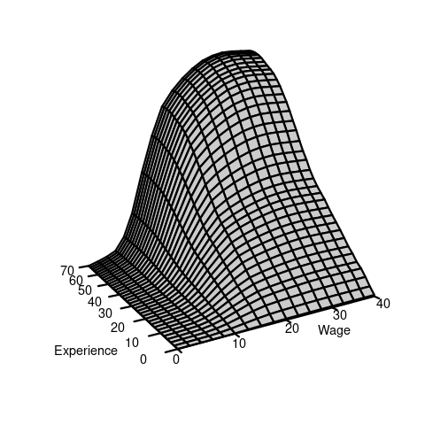
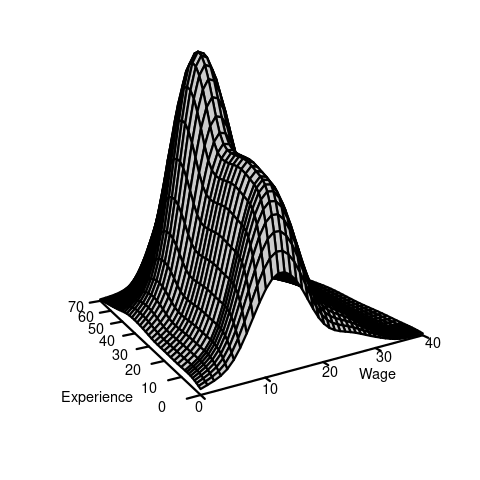
If F(a,b) is the joint CDF of (Y,Z), then the cross-moment is defined as: E[YZ] = \int_{-\infty}^\infty \int_{-\infty}^\infty ab \ \text{d}F(a,b). \tag{6.1} If Y and Z are continuous and F(a,b) is differentiable, the joint probability density function (PDF) of (Y,Z): f(a,b) = \frac{\partial^2}{\partial a \partial b} F(a,b). This allows us to write the differential of the CDF as \text{d}F(a,b) = f(a,b) \ \text{d} a \ \text{d}b, and the cross-moment becomes: E[YZ] = \int_{-\infty}^\infty \int_{-\infty}^\infty ab \ \text{d}F(a,b) = \int_{-\infty}^\infty \int_{-\infty}^\infty ab f(a,b) \ \text{d} a \ \text{d}b. In the wage and experience example, we have the following joint CDF and joint PDF:
If Y and Z are discrete with joint PMF \pi(a,b) and support \mathcal Y, the cross moment is E[YZ] = \int_{-\infty}^\infty \int_{-\infty}^\infty ab \ \text{d}F(a,b) = \sum_{a \in \mathcal Y} \sum_{b \in \mathcal Y} ab \ \pi(a,b). If one variable is discrete and the other is continuous, the expectation involves a mixture of summation and integration.
In general, the expected value of any real valued function g(Y,Z) is given by E[g(X,Y)] = \int_{-\infty}^\infty \int_{-\infty}^\infty g(a,b) \ \text{d}F(a,b).
6.4 Covariance and correlation
The covariance of Y and Z is defined as:
Cov(Y,Z) = E[(Y- E[Y])(Z-E[Z])] = E[YZ] - E[Y]E[Z].
The covariance of Y with itself is the variance:
Cov(Y,Y) = Var[Y].
The variance of the sum of two random variables depends on the covariance:
Var[Y+Z] = Var[Y] + 2 Cov(Y,Z) + Var[Z]
The correlation of Y and Z is
Corr(Y,Z) = \frac{Cov(Y,Z)}{sd(Y) sd(Z)}
where sd(Y) and sd(Z) are the standard deviations of Y and Z, respectively.
Uncorrelated
Y and Z are uncorrelated if Corr(Y,Z) = 0, or, equivalently, if Cov(Y,Z) = 0.
If Y and Z are uncorrelated, then: \begin{align*} E[YZ] &= E[Y] E[Z] \\ Var[Y+Z] &= Var[Y] + Var[Z] \end{align*}
If Y and Z are independent and have finite second moments, they are uncorrelated. However, the reverse is not necessarily true; uncorrelated variables are not always independent.
6.5 Expectations for random vectors
These concepts generalize to any k-dimensional random vector \boldsymbol Z = (Z_1, \ldots, Z_k).
The expectation vector of \boldsymbol Z is: E[\boldsymbol Z] = \begin{pmatrix} E[Z_1] \\ \vdots \\ E[Z_k] \end{pmatrix}. The covariance matrix of \boldsymbol Z is: \begin{align*} Var[\boldsymbol Z] &= E[(\boldsymbol Z-E[\boldsymbol Z])(\boldsymbol Z-E[\boldsymbol Z])'] \\ &= \begin{pmatrix} Var[Z_1] & Cov(Z_1, Z_2) & \ldots & Cov(X_1, Z_k) \\ Cov(Z_2, Z_1) & Var[Z_2] & \ldots & Cov(Z_2, Z_k) \\ \vdots & \vdots & \ddots & \vdots \\ Cov(Z_k, Z_1) & Cov(Z_k, Z_2) & \ldots & Var[Z_k] \end{pmatrix} \end{align*}
For any random vector \boldsymbol Z, the covariance matrix Var[\boldsymbol Z] is symmetric and positive semi-definite.