cps = read.csv("cps.csv")
exper = cps$experience
wage = cps$wage
edu = cps$education
fem = cps$female2 Summary statistics
In statistics, a univariate dataset Y_1, \ldots, Y_n or a multivariate dataset \boldsymbol X_1, \ldots, \boldsymbol X_n is often called a sample. It typically represents observations collected from a larger population. The sample distribution indicates how the sample values are distributed across possible outcomes.
Summary statistics, such as the sample mean and sample variance, provide a concise representation of key characteristics of the sample distribution. These summary statistics are related to the sample moments of a dataset.
2.1 Sample moments
The r-th sample moment about the origin (also called the r-th raw moment) is defined as \overline{Y^r} = \frac{1}{n} \sum_{i=1}^n Y_i^r.
For example, the first sample moment (r=1) is the sample mean (arithmetic mean): \overline Y = \frac{1}{n} \sum_{i=1}^n Y_i. The sample mean is the most common measure of central tendency.
To compute the sample mean of a vector Y in R, use mean(Y) or alternatively sum(Y)/length(Y). The r-th sample moment can be calculated with mean(Y^r).
2.2 Central sample moments
The r-th central sample moment is the average of the r-th powers of the deviations from the sample mean: \frac{1}{n} \sum_{i=1}^n (Y_i - \overline Y)^r For example, the second central moment (r=2) is the sample variance: \widehat \sigma_Y^2 = \frac{1}{n} \sum_{i=1}^n (Y_i - \overline Y)^2 = \overline{Y^2} - \overline Y^2. The sample variance measures the spread or dispersion of the data around the sample mean.
The sample standard deviation is the square root of the sample variance: \widehat \sigma_Y = \sqrt{\widehat \sigma_Y^2} = \sqrt{\frac{1}{n} \sum_{i=1}^n (Y_i - \overline Y)^2} = \sqrt{\overline{Y^2} - \overline Y^2} It quantifies the typical deviation of data points from the sample mean in the original units of measurement.
2.3 Degree of freedom corrections
When computing the sample mean \overline Y, we have n degrees of freedom because all data points Y_1, \ldots, Y_n can vary freely.
When computing variances, we take the sample mean of the squared deviations (Y_1 - \overline Y)^2, \ldots, (Y_n - \overline Y)^2. These elements cannot vary freely because \overline Y is computed from the same sample and implies the constraint \frac{1}{n} \sum_{i=1}^n (Y_i - \overline{Y}) = 0.
This means that the deviations are connected by this equation and are not all free to vary. Knowing the first n-1 of the deviations determines the last one: (Y_n - \overline Y) = - \sum_{i=1}^{n-1} (Y_i - \overline Y). Therefore, only n-1 deviations can vary freely, which results in n-1 degrees of freedom for the sample variance.
Because \sum_{i=1}^{n} (Y_i - \overline Y)^2 effectively contains only n-1 freely varying summands, it is common to account for this fact. The adjusted sample variance uses n−1 in the denominator: s_Y^2 = \frac{1}{n-1} \sum_{i=1}^n (Y_i - \overline Y)^2. The adjusted sample variance relates to the unadjusted sample variance as: s_Y^2 = \frac{n}{n-1} \widehat \sigma_Y^2. The adjusted sample standard deviation is: s_Y = \sqrt{\frac{1}{n-1} \sum_{i=1}^n (Y_i - \overline Y)^2} = \sqrt{\frac{n}{n-1}} \widehat \sigma_Y.
To compute the sample variance and sample standard deviation of a vector Y in R, use mean(Y^2)-mean(Y)^2 and sqrt(mean(Y^2)-mean(Y)^2), respectively. The built-in functions var(Y) and sd(Y) compute their adjusted versions.
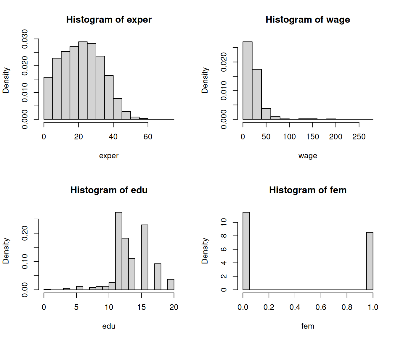
Let’s compute the sample means, sample variances, and adjusted sample variances of some variables from the cps dataset.
[1] 22.2082496 23.9026619 13.9246187 0.4257223[1] 136.0571603 428.9398785 7.5318408 0.2444828[1] 136.0598417 428.9483320 7.5319892 0.24448762.4 Histogram
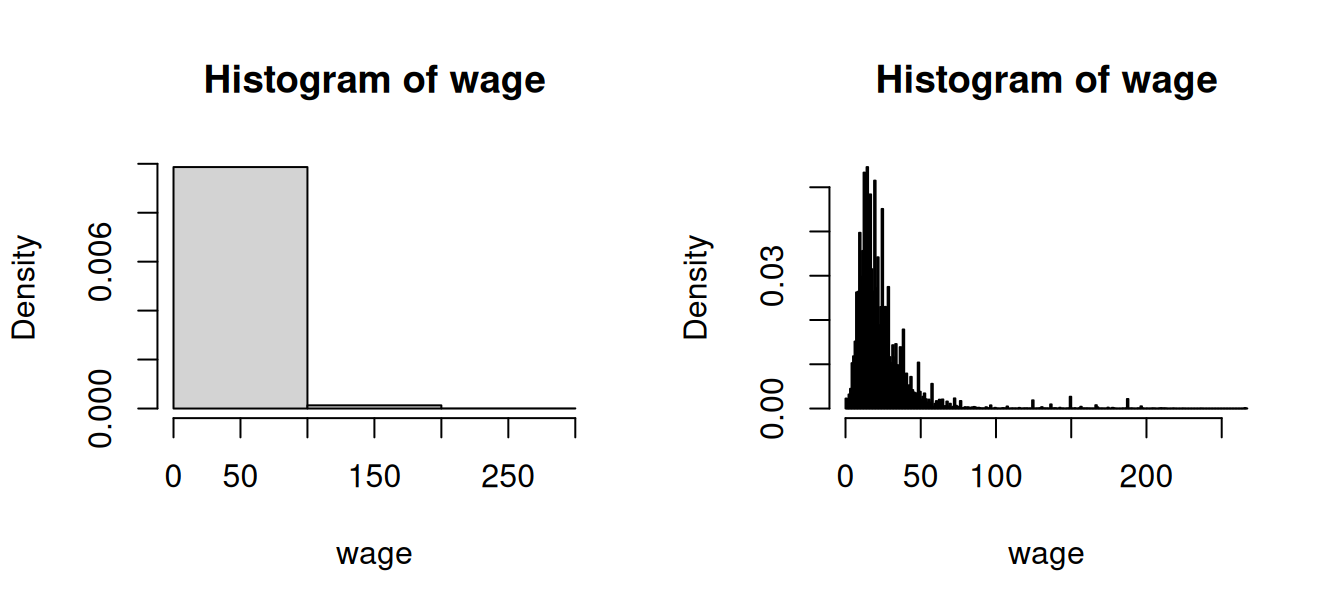
Histograms offer an intuitive visual representation of the sample distribution of a variable. A histogram divides the data range into B bins, each of equal width h, and counts the number of observations n_j within each bin. The height of the histogram at a in the j-th bin is \widehat f(a) = \frac{n_j}{nh}. The histogram is the plot of these heights, displayed as rectangles, with their area normalized so that the total area equals 1.
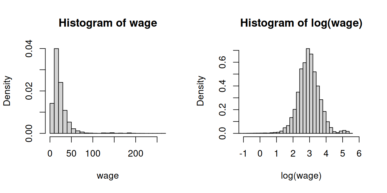
Running hist(wage, probability=TRUE) automatically selects a suitable number of bins B. Note that hist(wage) will plot absolute frequencies instead of relative ones. The shape of a histogram depends on the choice of B. You can experiment with different values using the breaks option:
2.5 Standardized sample moments
The r-th standardized sample moment is the central moment normalized by the sample standard deviation raised to the power of r. It is defined as: \frac{1}{n} \sum_{i=1}^n \bigg(\frac{Y_i - \overline Y}{\widehat \sigma_Y}\bigg)^r
2.5.1 Skewness
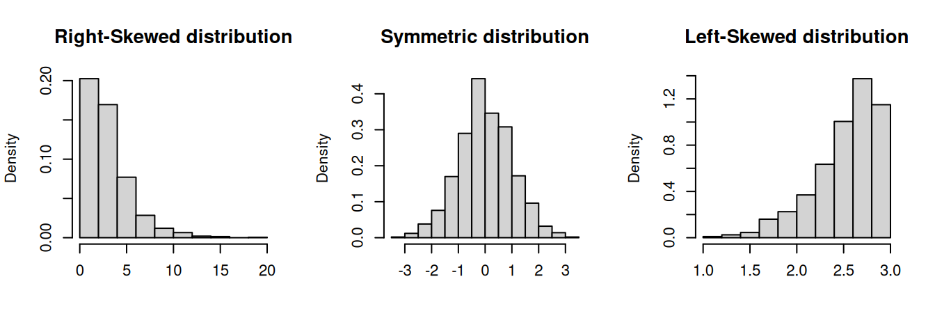
For example, the third standardized sample moment (r=3) is the sample skewness: \widehat{ske} = \frac{1}{n \widehat \sigma_Y^3} \sum_{i=1}^n (Y_i - \overline Y)^3. The skewness is a measure of asymmetry around the mean. A positive skewness indicates that the distribution has a longer or heavier tail on the right side (right-skewed), while a negative skewness indicates a longer or heavier tail on the left side (left-skewed). A perfectly symmetric distribution, such as the normal distribution, has a skewness of 0.
To compute the sample skewness in R, use:
For convenience, you can use the skewness(Y) function from the moments package, which performs the same calculation.
[1] 0.1872222 4.3201570 -0.2253251 0.3004446Wages are right-skewed because a few very rich individuals earn much more than the many with low to medium incomes. The other variables do not indicate any pronounced skewness.
2.5.2 Kurtosis
The sample kurtosis is the fourth standardized sample moment (r=4): \widehat{kur} = \frac{1}{n \widehat \sigma_Y^4} \sum_{i=1}^n (Y_i - \overline Y)^4.
Kurtosis measures the “tailedness” or heaviness of the tails of a distribution and can indicate the presence of extreme outliers. The reference value of kurtosis is 3, which corresponds to the kurtosis of a normal distribution. Values greater than 3 suggest heavier tails, while values less than 3 indicate lighter tails.
To compute the sample kurtosis in R, use:
For convenience, you can use the kurtosis(Y) function from the moments package, which performs the same calculation.
[1] 2.373496 30.370331 4.498264 1.090267The variable wage exhibits heavy tails due to a few super-rich outliers in the sample. In contrast, fem has light tails because there are approximately equal numbers of women and men.
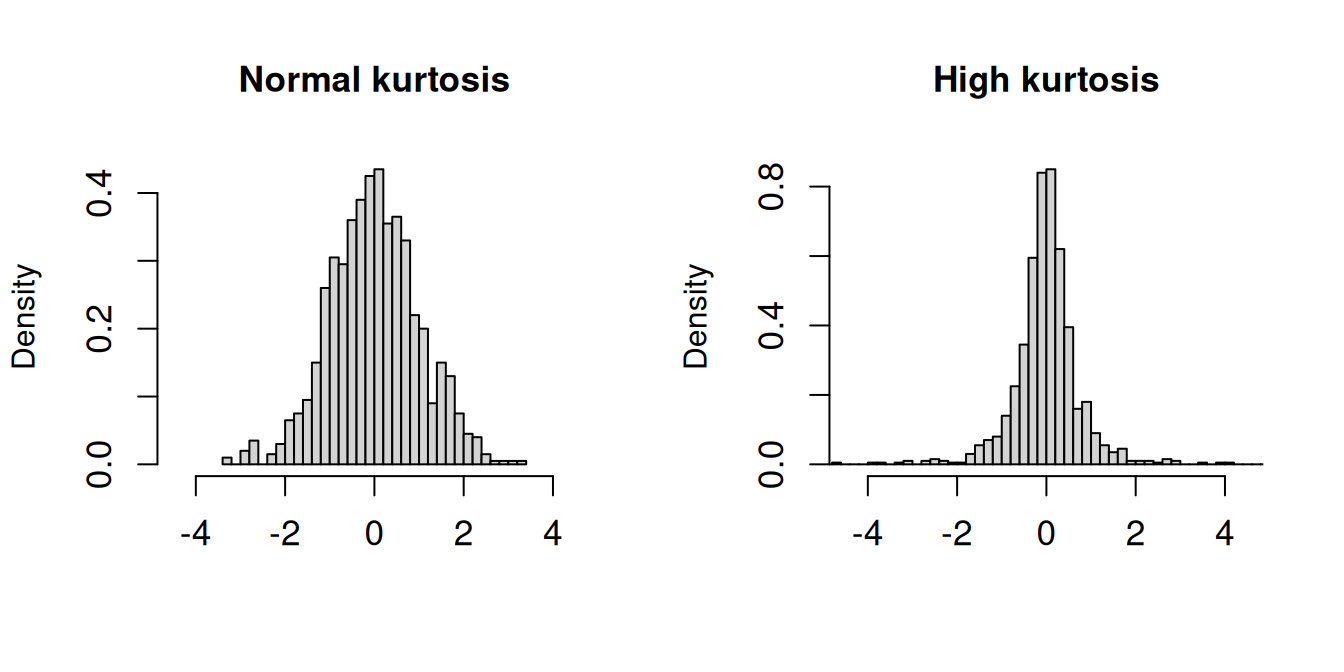
The plots display histograms of two standardized datasets (both have a sample mean of 0 and a sample variance of 1). The left dataset has a normal sample kurtosis (around 3), while the right dataset has a high sample kurtosis with heavier tails.
Some statistical software reports the excess kurtosis, which is defined as \widehat{kur} - 3. This shifts the reference value to 0 (instead of 3), making it easier to interpret: positive values indicate heavier tails than the normal distribution, while negative values indicate lighter tails. For example, the normal distribution has an excess kurtosis of 0.
2.5.3 Log-transformations
Right-skewed, heavy-tailed variables are common in real-world datasets, such as income levels, wealth accumulation, property values, insurance claims, and social media follower counts. A common transformation to reduce skewness and kurtosis in data is to use the natural logarithm:
In econometrics, statistics, and many programming languages including R, \log(\cdot) is commonly used to denote the natural logarithm (base e).
Note: On a pocket calculator, use LN to calculate the natural logarithm \log(\cdot)=\log_e(\cdot). If you use LOG, you will calculate the logarithm with base 10, i.e., \log_{10}(\cdot), which will give you a different result. The relationship between these logarithms is \log_{10}(x) = \log_{e}(x)/\log_{e}(10).
2.6 Sample cross moments
For a bivariate sample (Y_1, Z_1), \ldots, (Y_n, Z_n), we can compute cross moments that describe the relationship between the two variables. The (r,s)-th sample cross moment is defined as:
\overline{Y^rZ^s} = \frac{1}{n} \sum_{i=1}^n Y_i^r Z_i^s.
The most important cross moment is the (1,1)-th sample cross moment, or simply the first sample cross moment:
\overline{YZ} = \frac{1}{n} \sum_{i=1}^n Y_i Z_i.
The central sample cross moments are defined as:
\frac{1}{n} \sum_{i=1}^n (Y_i - \overline{Y})^r(Z_i - \overline{Z})^s.
The (1,1)-th central sample cross moment leads to the sample covariance:
\widehat{\sigma}_{YZ} = \frac{1}{n} \sum_{i=1}^n (Y_i - \overline{Y})(Z_i - \overline{Z}) = \overline{YZ} - \overline{Y} \overline{Z}.
Similar to the univariate case, we can define the adjusted sample covariance:
s_{YZ} = \frac{1}{n-1} \sum_{i=1}^n (Y_i - \overline{Y})(Z_i - \overline{Z}) = \frac{n}{n-1}\widehat{\sigma}_{YZ}.
The sample correlation coefficient is the standardized sample covariance:
r_{YZ} = \frac{s_{YZ}}{s_Y s_Z} = \frac{\sum_{i=1}^n (Y_i - \overline{Y})(Z_i - \overline{Z})}{\sqrt{\sum_{i=1}^n (Y_i - \overline{Y})^2}\sqrt{\sum_{i=1}^n (Z_i - \overline{Z})^2}} = \frac{\widehat{\sigma}_{YZ}}{\widehat{\sigma}_Y \widehat{\sigma}_Z}.
To compute these quantities for a bivariate sample collected in the vectors Y and Z, use cov(Y,Z) for the adjusted sample covariance and cor(Y,Z) for the sample correlation.
2.7 Sample moment matrices
Consider a multivariate dataset \boldsymbol X_1, \ldots, \boldsymbol X_n, such as the following subset of the cps dataset:
dat = data.frame(wage, edu, fem)The sample mean vector \overline{\boldsymbol X} contains the sample means of the k variables and is defined as \overline{\boldsymbol X} = \frac{1}{n} \sum_{i=1}^n \boldsymbol X_i.
colMeans(dat) wage edu fem
23.9026619 13.9246187 0.4257223 2.7.1 Sample covariance matrix
The sample covariance matrix \widehat{\Sigma} is the k \times k matrix given by \widehat{\Sigma} = \frac{1}{n} \sum_{i=1}^n (\boldsymbol X_i - \overline{\boldsymbol X})(\boldsymbol X_i - \overline{\boldsymbol X})'. Its elements \widehat \sigma_{h,l} represent the pairwise sample covariance between variables h and l: \widehat \sigma_{h,l} = \frac{1}{n} \sum_{i=1}^n (X_{ih} - \overline{X_h})(X_{il} - \overline{X_l}), \quad \overline{X_h} = \frac{1}{n} \sum_{i=1}^n X_{ih}.
The adjusted sample covariance matrix S is defined as S = \frac{1}{n-1} \sum_{i=1}^n (\boldsymbol X_i - \overline{\boldsymbol X})(\boldsymbol X_i - \overline{\boldsymbol X})' Its elements s_{h,l} are the adjusted sample covariances, with main diagonal elements s_{h}^2 = s_{h,h} being the adjusted sample variances: s_{h,l} = \frac{1}{n-1} \sum_{i=1}^n (X_{ih} - \overline{X_h})(X_{il} - \overline{X_l}).
cov(dat) wage edu fem
wage 428.948332 21.82614057 -1.66314777
edu 21.826141 7.53198925 0.06037303
fem -1.663148 0.06037303 0.244487642.7.2 Sample correlation matrix
The sample correlation coefficient between the variables h and l is the standardized sample covariance: r_{h,l} = \frac{s_{h,l}}{s_h s_l} = \frac{\sum_{i=1}^n (X_{ih} - \overline{X_h})(X_{il} - \overline{X_l})}{\sqrt{\sum_{i=1}^n (X_{ih} - \overline{X_h})^2}\sqrt{\sum_{i=1}^n (X_{il} - \overline{X_l})^2}} = \frac{\widehat \sigma_{h,l}}{\widehat \sigma_h \widehat \sigma_l}. These coefficients form the sample correlation matrix R, expressed as:
R = D^{-1} S D^{-1}, where D is the diagonal matrix of adjusted sample standard deviations: D = diag(s_1, \ldots, s_k) = \begin{pmatrix} s_1 & 0 & \ldots & 0 \\ 0 & s_2 & \ldots & 0 \\ \vdots & & \ddots & \vdots \\ 0 & 0 & \ldots & s_k \end{pmatrix} The matrices \widehat{\Sigma}, S, and R are symmetric.
cor(dat) wage edu fem
wage 1.0000000 0.38398973 -0.16240519
edu 0.3839897 1.00000000 0.04448972
fem -0.1624052 0.04448972 1.00000000We find a strong positive correlation between wage and edu, a substantial negative correlation between wage and fem, and a negligible correlation between edu and fem.