| ISCED level | Education level | Years of schooling |
|---|---|---|
| 1 | Primary | 4 |
| 2 | Lower Secondary | 10 |
| 3 | Upper secondary | 12 |
| 4 | Post-Secondary | 13 |
| 5 | Short-Cycle Tertiary | 14 |
| 6 | Bachelor's | 16 |
| 7 | Master's | 18 |
| 8 | Doctoral | 21 |
4 Probability
4.1 Random Sampling
From an empirical perspective, a dataset Y_1, \ldots, Y_n or \boldsymbol X_1, \ldots, \boldsymbol X_n is just a fixed array of numbers. Any summary statistic we compute – like a sample mean, sample correlation, or OLS coefficient – is simply a function of these numbers.
These statistics provide a snapshot of the data at hand but do not automatically reveal broader insights about the world. To add deeper meaning to these numbers, identify dependencies, and understand causalities, we must consider how the data were obtained.
A random experiment is an experiment whose outcome cannot be predicted with certainty. In statistical theory, any dataset is viewed as the result of such a random experiment.
The gender of the next person you meet, daily fluctuations in stock prices, monthly music streams of your favorite artist, or the annual number of pizzas consumed – all involve a certain amount of randomness and emerge from random experiments.
Sampling is the process of drawing observations from a population. Hence, a dataset is also called a sample. Each summary statistic, such as a sample mean or OLS coefficient, is one possible outcome of the random experiment. Repeating the experiment produces a new sample and new statistics.
In statistical theory, the population from which we draw observations is treated as infinite. It serves as a theoretical construct that includes not only existing members of a physical population, but all possible future or hypothetical individuals. In coin flip studies, for example, the infinite population represents not just all coin flips ever performed, but all possible coin flips that could theoretically occur in any context at any time.
The goal of statistical inference is to learn about the world from the observed sample. This requires assumptions about how the data were collected.
The simplest ideal assumption is random sampling, where each observation is drawn independently from the population – like drawing balls from an urn or randomly selecting survey participants. This principle is often called i.i.d. sampling (independent and identically distributed sampling). To define these concepts rigorously, we rely on probability theory.
4.2 Random variables
A random variable is a numerical summary of a random experiment. An outcome is a specific result of a random experiment. The sample space S is the set/collection of all potential outcomes.
Let’s consider some examples:
- Coin toss: The outcome of a coin toss can be “heads” or “tails”. This random experiment has a two-element sample space: S = \{heads, tails\}. We can express the experiment as a binary random variable: Y = \begin{cases} 1 & \text{if outcome is heads,} \\ 0 & \text{if outcome is tails.} \end{cases}
- Gender: If you conduct a survey and interview a random person to ask them about their gender, the answer may be “female”, “male”, or “diverse”. It is a random experiment since the person to be interviewed is selected randomly. The sample space has three elements: S = \{female, male, diverse\}. To focus on female vs. non-female, we can define the female dummy variable: Y = \begin{cases} 1 & \text{if the person is female,} \\ 0 & \text{if the person is not female.} \end{cases} Similarly, dummy variables for male and diverse can be defined.
- Education level: If you ask a random person about their education level according to the ISCED-2011 framework, the outcome may be one of the eight ISCED-2011 levels. We have an eight-element sample space: S = \{Level \ 1, Level \ 2, Level \ 3, Level \ 4, Level \ 5, Level \ 6, Level \ 7, Level \ 8\}. The eight-element sample space of the education-level random experiment provides a natural ordering. We define the random variable education as the number of years of schooling of the interviewed person: Y = \text{years of schooling} \in \{4, 10, 12, 13, 14, 16, 18, 21\}.
- Wage: If you ask a random person about their income per working hour in EUR, there are infinitely many potential answers. Any (non-negative) real number may be an outcome. The sample space is a continuum of different wage levels. The wage level of the interviewed is already numerical. The random variable is Y = \text{income per working hour in EUR}.
Random variables share the characteristic that their value is uncertain before conducting a random experiment (e.g., flipping a coin or selecting a random person for an interview). Their value is always a real number and is determined only once the experiment’s outcome is known.
4.3 Events and probabilities
An event of a random variable Y is a specific subset of the real line. Any real number defines an event (elementary event), and any open, half-open, or closed interval represents an event as well.
Let’s define some specific events:
- Elementary events: A_1 = \{Y=0\}, \quad A_2 = \{Y=1\}, \quad A_3 = \{Y=2.5\}
- Half-open events: \begin{align*} A_4 &= \{Y \geq 0\} = \{ Y \in [0,\infty) \} \\ A_5 &= \{ -1 \leq Y < 1 \} = \{ Y \in [-1,1) \}. \end{align*}
The probability function P assigns values between 0 and 1 to events. For a fair coin toss it is natural to assign the following probabilities: P(A_1) = P(Y=0) = 0.5, \quad P(A_2) = P(Y=1) = 0.5 By definition, the coin variable will never take the value 2.5, so we assign P(A_3) = P(Y=2.5) = 0. To assign probabilities to interval events, we check whether the events \{Y=0\} and/or \{Y=1\} are subsets of the event of interest.
If both \{Y=0\} and \{Y=1\} are contained in the event of interest, the probability is 1. If only one of them is contained, the probability is 0.5. If neither is contained, the probability is 0. P(A_4) = P(Y \geq 0) = 1, \quad P(A_5) = P( -1 \leq Y < 1) = 0.5.
Every event has a complementary event, and for any pair of events we can take the union and intersection. Let’s define further events:
- Complements: A_6 = A_4^c = \{Y \geq 0\}^c = \{ Y < 0\} = \{Y \in (-\infty, 0)\},
- Unions: A_7 = A_1 \cup A_6 = \{Y=0\} \cup \{Y< 0\} = \{Y \leq 0\}
- Intersections: A_8 = A_4 \cap A_5 = \{Y \geq 0\} \cap \{ -1 \leq Y < 1 \} = \{ 0 \leq Y < 1 \}
- Iterations of it: A_9 = A_1 \cup A_2 \cup A_3 \cup A_5 \cup A_6 \cup A_7 \cup A_8 = \{ Y \in (-\infty, 1] \cup \{2.5\}\},
- Certain event: A_{10} = A_9 \cup A_9^c = \{Y \in (-\infty, \infty)\} = \{Y \in \mathbb R\}
- Empty event: A_{11} = A_{10}^c = \{ Y \notin \mathbb R \} = \{ \}
You may verify that P(A_1) = 0.5, P(A_2) = 0.5, P(A_3) = 0, P(A_4) = 1 P(A_5) = 0.5, P(A_6) = 0, P(A_7) = 0.5, P(A_8) = 0.5, P(A_9) = 1, P(A_{10}) = 1, P(A_{11}) = 0 for the coin toss experiment.
4.4 Probability function
The probability function P assigns probabilities to events. The set of all events for which probabilities can be assigned is called the Borel sigma-algebra, denoted as \mathcal B.
The previously mentioned events A_1, \ldots, A_{11} are elements of \mathcal B. Any event of the form \{ Y \in (a,b) \} with a, b \in \mathbb{R} is also in \mathcal B. Moreover, \mathcal B includes all possible unions, intersections, and complements of these events. Essentially, it represents the complete collection of events for which we would ever compute probabilities in practice.
A probability function P must satisfy certain fundamental rules (axioms) to ensure a well-defined probability framework:
Basic rules of probability
- P(A) \geq 0 for any event A
- P(Y \in \mathbb R) = 1 for the certain event
- P(A \cup B) = P(A) + P(B) if A and B are disjoint
- P(Y \notin \mathbb R) = 0 for the empty event
- 0 \leq P(A) \leq 1 for any event A
- P(A) \leq P(B) if A is a subset of B
- P(A^c) = 1 - P(A) for the complement event of A
- P(A \cup B) = P(A) + P(B) - P(A \cap B) for any events A, B
Two events A and B are disjoint if A \cap B = \{\}, meaning they have no common outcomes. For instance, A_1 = \{Y=0\} and A_2 = \{Y=1\} are disjoint. However, A_1 and A_4 = \{Y \geq 0\} are not disjoint because their intersection, A_1 \cap A_4 = \{Y=0\}, is nonempty.
The first three properties listed above are known as the axioms of probability. The remaining properties follow as logical consequences of these axioms.
4.5 Distribution function
Assigning probabilities to events is straightforward for binary variables, like coin tosses. For instance, knowing that P(Y = 1) = 0.5 allows us to derive the probabilities for all events in \mathcal B. However, for more complex variables, such as education or wage, defining probabilities for all possible events becomes more challenging due to the vast number of potential set operations involved.
Fortunately, it turns out that knowing the probabilities of events of the form \{Y \leq a\} is enough to determine the probabilities of all other events. These probabilities are summarized in the cumulative distribution function.
Cumulative distribution function (CDF)
The cumulative distribution function (CDF) of a random variable Y is F(a) := P(Y \leq a), \quad a \in \mathbb R.
The CDF is sometimes simply referred to as the distribution function, or the distribution.
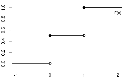
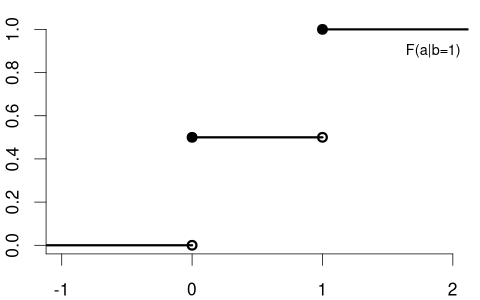
The cumulative distribution function (CDF) of the variable coin is F(a) = \begin{cases} 0 & a < 0, \\ 0.5 & 0 \leq a < 1, \\ 1 & a \geq 1, \end{cases} with the following CDF plot:
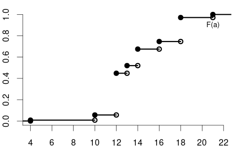
The CDF of the variable education could be
and the CDF of the variable wage may have the following form:
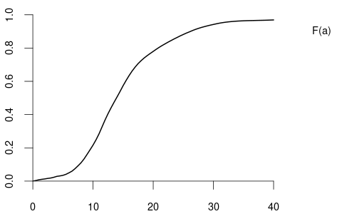
The CDF of a continuous random variable is smooth, while the CDF of a discrete random variable contains jumps and is flat between jumps. For example, variables like coin and education are discrete, whereas wage is continuous.
Any function F(a) with the following properties defines a valid probability distribution:
- Non-decreasing: F(a) \leq F(b) for a \leq b;
- Limits at 0 and 1: \displaystyle \lim_{a \to -\infty} F(a) = 0 and \displaystyle \lim_{a \to \infty} F(a) = 1
- Right-continuity: \displaystyle \lim_{\varepsilon \to 0, \varepsilon \geq 0} F(a + \varepsilon) = F(a)
Right-continuity ensures that cumulative probabilities include the probability at each point, which is especially important for discrete variables with their jump points.
The right-continuity property means that the CDF includes the probability mass at each point a, ensuring P(Y \leq a) includes P(Y = a). This property is particularly important for discrete random variables where there are jumps in the CDF.
By the basic rules of probability, we can compute the probability of any event of interest if we know the probabilities of all events of the forms \{Y \leq a\} and \{Y = a \}.
Some basic rules for the CDF (for a < b):
- P(Y \leq a) = F(a)
- P(Y > a) = 1 - F(a)
- P(Y < a) = F(a) - P(Y=a)
- P(Y \geq a) = 1 - P(Y < a)
- P(a < Y \leq b) = F(b) - F(a)
- P(a < Y < b) = F(b) - F(a) - P(Y=b)
- P(a \leq Y \leq b) = F(b) - F(a) + P(Y=a)
- P(a \leq Y < b) = P(a \leq Y \leq b) - P(Y=b)
A probability of the form P(Y=a), which involves only an elementary event, is called a point probability.
4.6 Probability mass function
The point probability P(Y = a) represents the size of the jump at a \in \mathbb{R} in the CDF F(a): P(Y=a) = F(a) - \lim_{\epsilon \to 0, \varepsilon \geq 0} F(a-\varepsilon), which is the jump height at a. We summarize the CDF jump heights or point probabilities in the probability mass function:
Probability mass function (PMF)
The probability mass function (PMF) of a random variable Y is \pi(a) := P(Y = a), \quad a \in \mathbb R
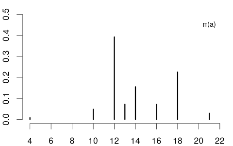
The PMF of the coin variable is \pi(a) = P(Y=a) = \begin{cases} 0.5 & \text{if} \ a \in\{0,1\}, \\ 0 & \text{otherwise}. \end{cases} The education variable may have the following PMF: \pi(a) = P(Y=a) = \begin{cases} 0.008 & \text{if} \ a = 4 \\ 0.048 & \text{if} \ a = 10 \\ 0.392 & \text{if} \ a = 12 \\ 0.072 & \text{if} \ a = 13 \\ 0.155 & \text{if} \ a = 14 \\ 0.071 & \text{if} \ a = 16 \\ 0.225 & \text{if} \ a = 18 \\ 0.029 & \text{if} \ a = 21 \\ 0 & \text{otherwise} \end{cases}
Because continuous variables have no jumps in their CDF, the PMF concept makes only sense for discrete random variables.
4.7 Probability density function
For continuous random variables, the CDF has no jumps, meaning the probability of any specific value is zero, and probability is distributed continuously over intervals. Unlike discrete random variables, which are characterized by both the PMF and the CDF, continuous variables do not have a positive PMF. Instead, they are described by the probability density function (PDF), which serves as the continuous analogue. If the CDF is differentiable, the PDF is given by its derivative:
Probability density function
The probability density function (PDF) or simply density function of a continuous random variable Y is the derivative of its CDF: f(a) = \frac{d}{da} F(a). Conversely, the CDF can be obtained from the PDF by integration: F(a) = \int_{-\infty}^a f(u) \ \text{d}u
Any function f(a) with the following properties defines a valid probability density function:
- Non-negativity: f(a) \geq 0 for all a \in \mathbb R;
- Normalization: \int_{-\infty}^\infty f(u) \ \text{d}u = 1.
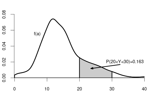
Basic rules for continuous random variables (with a \leq b):
- \displaystyle P(Y = a) = \int_a^a f(u) \ \text{d}u = 0
- \displaystyle P(Y \leq a) = P(Y < a) = F(a) = \int_{-\infty}^a f(u) \ \text{d}u
- \displaystyle P(Y > a) = P(Y \geq a) = 1 - F(a) = \int_a^\infty f(u) \ \text{d}u
- \displaystyle P(a < Y < b) = F(b) - F(a) = \int_a^b f(u) \ \text{d}u
- \displaystyle P(a < Y < b) = P(a < Y \leq b) = P(a \leq Y \leq b) = P(a \leq Y < b)
4.8 Conditional distribution
The distribution of wage may differ between men and women. Similarly, the distribution of education may vary between married and unmarried individuals. In contrast, the distribution of a coin flip should remain the same regardless of whether the person tossing the coin earns 15 or 20 EUR per hour.
The conditional cumulative distribution function (conditional CDF), F_{Y|Z=b}(a) = F_{Y|Z}(a|b) = P(Y\leq a|Z=b), represents the distribution of a random variable Y given that another random variable Z takes a specific value b. It answers the question: “If we know that Z=b, what is the distribution of Y?”
For example, suppose that Y represents wage and Z represents education
- F_{Y|Z=12}(a) is the CDF of wages among individuals with 12 years of education.
- F_{Y|Z=14}(a) is the CDF of wages among individuals with 14 years of education.
- F_{Y|Z=18}(a) is the CDF of wages among individuals with 18 years of education.
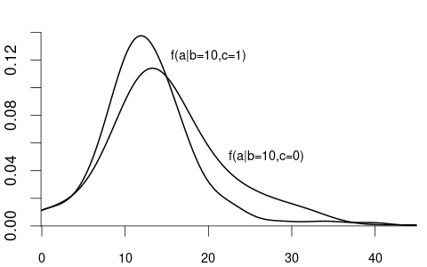
Since wage is a continuous variable, its conditional distribution given any specific value of another variable is also continuous. The conditional density of Y given Z=b is defined as the derivative of the conditional CDF: f_{Y|Z=b}(a) = f_{Y|Z}(a|b) = \frac{d}{d a} F_{Y|Z=b}(a).
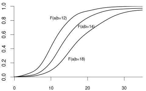
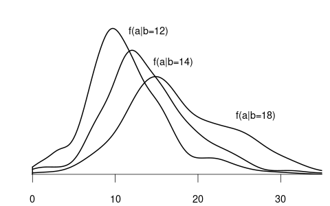
We observe that the distribution of wage varies across different levels of education. For example, individuals with fewer years of education are more likely to earn less than 20 EUR per hour: P(Y\leq 20 | Z=12) = F_{Y|Z=12}(20) > F_{Y|Z=18}(20) = P(Y\leq 20|Z = 18). Because the conditional distribution of Y given Z=b depends on the value of Z=b we say that the random variables Y and Z are dependent random variables.
Note that the conditional CDF F_{Y|Z=b}(a) can only be defined for events Z=b that are possible, i.e. b must be in the support of Z. Formally, the support consists of all b \in \mathbb R where the cumulative distribution function F_Z(b) is not flat – meaning it either increases continuously or has a jump. For instance, the support of the variable education is \{4, 10, 12, 13, 14, 16, 18, 21\} and the support of the variable wage is \{a \in \mathbb R: a \geq 0\}.
We can also condition on more than one variable. Let Z_1 represent the labor market experience in years and Z_2 be the female dummy variable. The conditional CDF of Y given Z_1 = b and Z_2 = c is: F_{Y|Z_1=b,Z_2=c}(a) = F_{Y|Z_1,Z_2}(a|b,c) = P(Y \leq a|Z_1=b, Z_2=c).
For example:
- F_{Y|Z_1=10,Z_2=1}(a) is the CDF of wages among women with 10 years of experience.
- F_{Y|Z_1=10,Z_2=0}(a) is the CDF of wages among men with 10 years of experience.
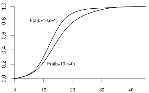
Clearly the random variable Y and the random vector (Z_1, Z_2) are dependent.
More generally, we can condition on the event that a k-variate random vector \boldsymbol Z = (Z_1, \ldots, Z_k)' takes the value \{\boldsymbol Z = \boldsymbol b\}, i.e. \{Z_1 = b_1, \ldots, Z_k = b_k\}. The conditional CDF of Y given \{\boldsymbol Z = \boldsymbol b\} is F_{Y|\boldsymbol Z = \boldsymbol b}(a) = F_{Y|Z_1 = b_1, \ldots, Z_k = b_k}(a).
The variable of interest, Y, can also be discrete. Then, any conditional CDF of Y is also discrete. Below is the conditional CDF of education given the married dummy variable:
- F_{Y|Z=0}(a) is the CDF of education among unmarried individuals.
- F_{Y|Z=1}(a) is the CDF of education among married individuals.
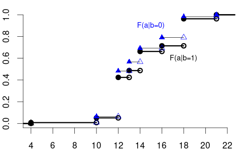
The conditional PMFs \pi_{Y|Z=0}(a) = P(Y = a | Z=0) and \pi_{Y|Z=1}(a)= P(Y = a | Z=1) indicate the jump heights of F_{Y|Z=0}(a) and F_{Y|Z=1}(a) at a.
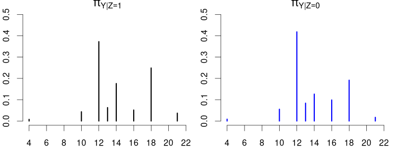
Clearly, education and married are dependent random variables. E.g., \pi_{Y|Z=0}(12) > \pi_{Y|Z=1}(12) and \pi_{Y|Z=0}(18) < \pi_{Y|Z=1}(18).
In contrast, consider Y= coin flip and Z= married dummy variable. The CDF of a coin flip should be the same for married or unmarried individuals:

Because F_Y(a) = F_{Y|Z=0}(a) = F_{Y|Z=1}(a) \quad \text{for all} \ a we say that Y and Z are independent random variables.
4.9 Independence of random variables
Independence
Y and Z are independent if and only if F_{Y|Z=b}(a) = F_{Y}(a) \quad \text{for all} \ a \quad \text{and for almost every} \ b.
Note that if F_{Y|Z=b}(a) = F_{Y}(a) for all b, then automatically F_{Z|Y=a}(b) = F_{Y}(b) for all a. Due to this symmetry we can equivalently define independence through the property F_{Z|Y=a}(b) = F_{Z}(b).
Here, “for almost every b” means for every b in the support of Z, apart from a set of values that has probability 0 under Z. Put differently, the condition must hold for all b-values that Z can actually take, with exceptions allowed only on a set whose probability is 0. Think of it as “for all practical purposes”. The condition must hold for all values b that could realistically occur. For instance, we only need independence to hold for non-negative wages. We don’t need to check independence for negative wages since they can’t occur.
The definition naturally generalizes to Z_1, Z_2, Z_3. They are mutually independent if, for each i \in \{1,2,3\}, the conditional distribution of Z_i given the other two equals its marginal distribution. In CDF form, this means:
- F_{Z_1|Z_2=b_2, Z_3=b_3}(a) = F_{Z_1}(a)
- F_{Z_2|Z_1=b_1, Z_3=b_3}(a) = F_{Z_2}(a)
- F_{Z_3|Z_1=b_1, Z_2=b_2}(a) = F_{Z_3}(a)
for all a and for almost every (b_1, b_2, b_3). Here, we need all three conditions.
Mutual independence
The random variables Z_1, \ldots, Z_n are mutually independent if and only if, for each i = 1,\dots,n, F_{Z_i | Z_1=b_1,\ldots,Z_{i-1}=b_{i-1},\,Z_{i+1}=b_{i+1},\ldots,Z_n=b_n}(a) = F_{Z_i}(a). for all a and almost every (b_1, \ldots, b_n).
An equivalent viewpoint uses the joint CDF of the vector \boldsymbol Z = (Z_1, \ldots, Z_n)', which is defined as: F_{\boldsymbol Z}(\boldsymbol a) = F_{Z_1, \ldots, Z_n}(a_1, \ldots, a_n) = P(Z_1 \leq a_1, \ldots, Z_n \leq a_n) = P(\boldsymbol Z \leq \boldsymbol a), where P(Z_1 \leq a_1, \ldots, Z_n \leq a_n) = P(\{Z_1 \leq a_1\} \cap \ldots \cap \{Z_n \leq a_n\}). Then Z_1, \ldots, Z_n are mutually independent if and only if the joint CDF is the product of the marginal CDFs: F_{\boldsymbol Z}(\boldsymbol a) = F_{Z_1}(a_1) \cdots F_{Z_n}(a_n) \quad \text{for all} \ a_1, \ldots, a_n.
4.10 Independence of random vectors
Often in practice, we work with multiple variables recorded for different individuals or time points. For example, consider two random vectors: \boldsymbol{X}_1 = (X_{11}, \ldots, X_{1k})', \quad \boldsymbol{X}_2 = (X_{21}, \ldots, X_{2k})'. The conditional distribution function of \boldsymbol{X}_1 given that \boldsymbol{X}_2 takes the value \boldsymbol{b}=(b_1,\ldots,b_k)' is F_{\boldsymbol{X}_1 | \boldsymbol{X}_2 = \boldsymbol{b}}(\boldsymbol{a}) = P(\boldsymbol{X}_1 \le \boldsymbol{a}|\boldsymbol{X}_2 = \boldsymbol{b}), where \boldsymbol{X}_1 \le \boldsymbol{a} means X_{1j} \le a_j for each coordinate j=1,\ldots,k.
For instance, if \boldsymbol{X}_1 and \boldsymbol{X}_2 represent the survey answers of two different, randomly chosen people, then F_{\boldsymbol{X}_2 | \boldsymbol{X}_1=\boldsymbol{b}}(\boldsymbol{a}) describes the distribution of the second person’s answers, given that the first person’s answers are \boldsymbol{b}. If the two people are truly randomly selected and unrelated to one another, we would not expect \boldsymbol{X}_2 to depend on whether \boldsymbol{X}_1 equals \boldsymbol{b} or some other value \boldsymbol{c}. In other words, knowing \boldsymbol X_1 provides no information that changes the distribution of \boldsymbol X_2.
Independence of random vectors
Two random vectors \boldsymbol{X}_1 and \boldsymbol{X}_2 are independent if and only if F_{\boldsymbol{X}_1 | \boldsymbol{X}_2 = \boldsymbol{b}}(\boldsymbol{a}) = F_{\boldsymbol{X}_1}(\boldsymbol{a}) \quad \text{for all } \boldsymbol{a} \quad \text{and for almost every } \boldsymbol{b}.
This definition extends naturally to mutual independence of n random vectors \boldsymbol{X}_1,\dots,\boldsymbol{X}_n, where \boldsymbol{X}_i = (X_{i1},\dots,X_{ik})'. They are called mutually independent if, for each i = 1,\dots,n, F_{\boldsymbol X_i| \boldsymbol X_1=\boldsymbol b_1, \ldots, \boldsymbol X_{i-1}=\boldsymbol b_{i-1}, \boldsymbol X_{i+1}=\boldsymbol b_{i+1}, \ldots, \boldsymbol X_n = \boldsymbol b_n}(\boldsymbol a) = F_{\boldsymbol X_i}(\boldsymbol a) for all \boldsymbol{a} and almost every (\boldsymbol{b}_1,\dots,\boldsymbol{b}_n).
Hence, in an independent sample, what the i-th randomly chosen person answers does not depend on anyone else’s answers.
i.i.d. sample / random sample
A collection of random vectors \boldsymbol{X}_1, \dots, \boldsymbol{X}_n is i.i.d. (independent and identically distributed) if they are mutually independent and have the same distribution function F. Formally, F_{\boldsymbol X_i| \boldsymbol X_1=\boldsymbol b_1, \ldots, \boldsymbol X_{i-1}=\boldsymbol b_{i-1}, \boldsymbol X_{i+1}=\boldsymbol b_{i+1}, \ldots, \boldsymbol X_n = \boldsymbol b_n}(\boldsymbol a) = F(\boldsymbol a) for all i=1, \ldots, n, for all \boldsymbol{a}, and almost all (\boldsymbol{b}_1,\dots,\boldsymbol{b}_n).
An i.i.d. dataset (or random sample) is one where each observation not only comes from the same population distribution F but is independent of the others. The function F is called the population distribution or the data-generating process (DGP).
The CPS data are cross-sectional data: n individuals are randomly selected from the U.S. population and independently interviewed on k variables. Consequently, these n observations form an i.i.d. sample.
If Y_1, \ldots, Y_n are i.i.d., then \log(Y_1), \ldots, \log(Y_n) are also i.i.d. In fact, any identical transformation of each observation preserves the independence and identical distribution. More formally, if \boldsymbol X_1, \ldots, \boldsymbol X_n is i.i.d., then g(\boldsymbol X_1), \ldots, g(\boldsymbol X_n) is i.i.d. as well, for any function g(\cdot). For instance, if the wages of n interviewed individuals are i.i.d., then their log-wages are also i.i.d.
Sampling methods of obtaining economic datasets that may be considered as random sampling are:
-
Survey sampling
Examples: representative survey of randomly selected households from a list of residential addresses; online questionnaire to a random sample of recent customers -
Administrative records
Examples: data from a government agency database, Statistisches Bundesamt, ECB, etc. -
Direct observation
Collected data without experimental control and interactions with the subject. Example: monitoring customer behavior in a retail store -
Web scraping
Examples: collected house prices on real estate sites or hotel/electronics prices on booking.com/amazon, etc. -
Field experiment
To study the impact of a treatment or intervention on a treatment group compared with a control group. Example: testing the effectiveness of a new teaching method by implementing it in a selected group of schools and comparing results to other schools with traditional methods -
Laboratory experiment
Example: a controlled medical trial for a new drug
Examples of cross-sectional data sampling that may produce some dependence across observations are:
Stratified sampling
The population is first divided into homogenous subpopulations (strata), and a random sample is obtained from each stratum independently. Examples: divide companies into industry strata (manufacturing, technology, agriculture, etc.) and sample from each stratum; divide the population into income strata (low-income, middle-income, high-income).
The sample is independent within each stratum, but it is not between different strata. The strata are defined based on specific characteristics that may be correlated with the variables collected in the sample.Clustered sampling
Entire subpopulations are drawn. Example: new teaching methods are compared to traditional ones on the student level, where only certain classrooms are randomly selected, and all students in the selected classes are evaluated.
Within each cluster (classroom), the sample is dependent because of the shared environment and teacher’s performance, but between classrooms, it is independent.
Other types of data we often encounter in econometrics are time series data, panel data, or spatial data:
Time series data consists of observations collected at different points in time, such as stock prices, daily temperature measurements, or GDP figures. These observations are ordered and typically show temporal trends, seasonality, and autocorrelation.
Panel data involves observations collected on multiple entities (e.g., individuals, firms, countries) over multiple time periods. Every entity thus forms a cluster, within which there is a time series of observations. In this sense, panel data is a specific form of clustered sampling.
Spatial data includes observations taken at different geographic locations, where values at nearby locations are often correlated.
Time series, panel, and spatial data cannot be considered a random sample given their temporal or geographic dependence.